决策树
用于分类和回归的非监督学习方法,通过简单的决策规则(if-else)预测目标
优缺点
- 思想简单,可视乎表达,易理解,可以处理多分类问题
- 可能会过拟合,此时需要剪枝、采用设置最小样本数目或树的深度
- 基于启发式算法,节点采用贪婪算法(局部最优),不能保证全局最优,可以随机抽取样本,训练多个树
- 过于复杂的概念,无法表达
决策树 CART
CART: classifcation and regression tree
irsi数据集构建分类决策树
from sklearn.datasets import load_iris
from sklearn import tree

#加载iris数据集
iris = load_iris()
clf = tree.DecisionTreeClassifier()
clf = clf.fit(iris.data, iris.target)
import pydotplus
dot_data = tree.export_graphviz(clf, out_file=None)
#dot_data = tree.export_graphviz(clf, out_file=None,
                              feature_names=iris.feature_names,
                              class_names=iris.target_names,
                              filled=True, rounded=True,
                              special_characters=True)
graph = pydotplus.graph_from_dot_data(dot_data)
#导出决策树
graph.write_pdf(“iris.pdf”)
#Image(graph.create_png())

sklearn example
import numpy as np
import matplotlib.pyplot as plt
from sklearn.datasets import load_iris
from sklearn.tree import DecisionTreeClassifier
Parameters
n_classes = 3
plot_colors = “ryb”
plot_step = 0.02
Load data
iris = load_iris()
for pairidx, pair in enumerate([[0, 1], [0, 2], [0, 3],
[1, 2], [1, 3], [2, 3]]):
# We only take the two corresponding features
X = iris.data[:, pair]
y = iris.target
# Train
clf = DecisionTreeClassifier().fit(X, y)
Plot the decision boundary
plt.subplot(2, 3, pairidx + 1)
x_min, x_max = X[:, 0].min() - 1, X[:, 0].max() + 1
y_min, y_max = X[:, 1].min() - 1, X[:, 1].max() + 1
xx, yy = np.meshgrid(np.arange(x_min, x_max, plot_step),
np.arange(y_min, y_max, plot_step))
plt.tight_layout(h_pad=0.5, w_pad=0.5, pad=2.5)
Z = clf.predict(np.c_[xx.ravel(), yy.ravel()])
Z = Z.reshape(xx.shape)
cs = plt.contourf(xx, yy, Z, cmap=plt.cm.RdYlBu)
plt.xlabel(iris.feature_names[pair[0]])
plt.ylabel(iris.feature_names[pair[1]])
Plot the training points
for i, color in zip(range(n_classes), plot_colors):
idx = np.where(y == i)
plt.scatter(X[idx, 0], X[idx, 1], c=color, label=iris.target_names[i],
cmap=plt.cm.RdYlBu, edgecolor=’black’, s=15)
plt.suptitle(“Decision surface of a decision tree using paired features”)
plt.legend(loc=’lower right’, borderpad=0, handletextpad=0)
plt.axis(“tight”)
plt.show()

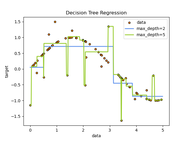
决策树回归
max_depth:图的深度,值太大会导致过拟合
# Import the necessary modules and libraries
import numpy as np
from sklearn.tree import DecisionTreeRegressor
import matplotlib.pyplot as plt
Create a random dataset
rng = np.random.RandomState(1)
X = np.sort(5 * rng.rand(80, 1), axis=0)
y = np.sin(X).ravel() #学习sin曲线
y[::5] += 3 * (0.5 - rng.rand(16)) #干扰值
Fit regression model
regr_1 = DecisionTreeRegressor(max_depth=2)
regr_2 = DecisionTreeRegressor(max_depth=5)
regr_1.fit(X, y)
regr_2.fit(X, y)
Predict
X_test = np.arange(0.0, 5.0, 0.01)[:, np.newaxis]
y_1 = regr_1.predict(X_test)
y_2 = regr_2.predict(X_test)
Plot the results
plt.figure()
plt.scatter(X, y, s=20, edgecolor=”black”,
c=”darkorange”, label=”data”)
plt.plot(X_test, y_1, color=”cornflowerblue”,
label=”max_depth=2”, linewidth=2)
plt.plot(X_test, y_2, color=”yellowgreen”, label=”max_depth=5”, linewidth=2)
plt.xlabel(“data”)
plt.ylabel(“target”)
plt.title(“Decision Tree Regression”)
plt.legend()
plt.show()
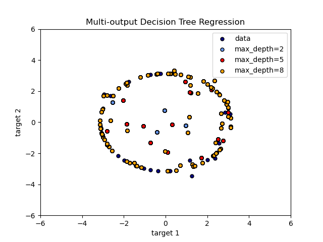
多输出问题
import numpy as np
import matplotlib.pyplot as plt
from sklearn.tree import DecisionTreeRegressor
Create a random dataset
rng = np.random.RandomState(1)
X = np.sort(200 * rng.rand(100, 1) - 100, axis=0)
y = np.array([np.pi * np.sin(X).ravel(), np.pi * np.cos(X).ravel()]).T #输出X正弦 余弦
y[::5, :] += (0.5 - rng.rand(20, 2)) #干扰
Fit regression model
regr_1 = DecisionTreeRegressor(max_depth=2)
regr_2 = DecisionTreeRegressor(max_depth=5)
regr_3 = DecisionTreeRegressor(max_depth=8)
regr_1.fit(X, y)
regr_2.fit(X, y)
regr_3.fit(X, y)
Predict
X_test = np.arange(-100.0, 100.0, 0.01)[:, np.newaxis]
y_1 = regr_1.predict(X_test)
y_2 = regr_2.predict(X_test)
y_3 = regr_3.predict(X_test)
Plot the results
plt.figure()
s = 25
plt.scatter(y[:, 0], y[:, 1], c=”navy”, s=s,
edgecolor=”black”, label=”data”)
plt.scatter(y_1[:, 0], y_1[:, 1], c=”cornflowerblue”, s=s,
edgecolor=”black”, label=”max_depth=2”)
plt.scatter(y_2[:, 0], y_2[:, 1], c=”red”, s=s,
edgecolor=”black”, label=”max_depth=5”)
plt.scatter(y_3[:, 0], y_3[:, 1], c=”orange”, s=s,
edgecolor=”black”, label=”max_depth=8”)
plt.xlim([-6, 6])
plt.ylim([-6, 6])
plt.xlabel(“target 1”)
plt.ylabel(“target 2”)
plt.title(“Multi-output Decision Tree Regression”)
plt.legend(loc=”best”)
plt.show()